dirk
Inferring correlation from pairs
In this article we briefly look at the transitivity of correlation. This means if we know that pairs (x, y) and (y, z) are positively correlated what can we say about correlation of (x, z).
This is a bit like filling in missing values in a correlation matrix.
It has been proven that
$\rho(x, y) = a$ and $\rho(y, z) = b$
implies
$ab - \sqrt{(1 - a^2)(1 - b^2)} \le \rho(x, z) \le ab + \sqrt{(1 - a^2)(1 - b^2)}$
So we can say what are the lower and upper bounds for the (x, z) correlation.
If we know these bounds can we than overlay a prior distribution to visualise the density of that correlation estimate.
We will use the maxent function in preliz to derive this distribution.
Assume we know correlations 0.5 and 0.6 and we want to infer the missing one. The range is (-.39, .99).
a = .6
b = .5
lb = a * b - np.sqrt((1 - a ** 2) * (1 - b ** 2))
ub = a * b + np.sqrt((1 - a ** 2) * (1 - b ** 2))
lb, ub
(-0.39282032302755093, 0.992820323027551)
The mid point of that range is 0.3, which is a * b.
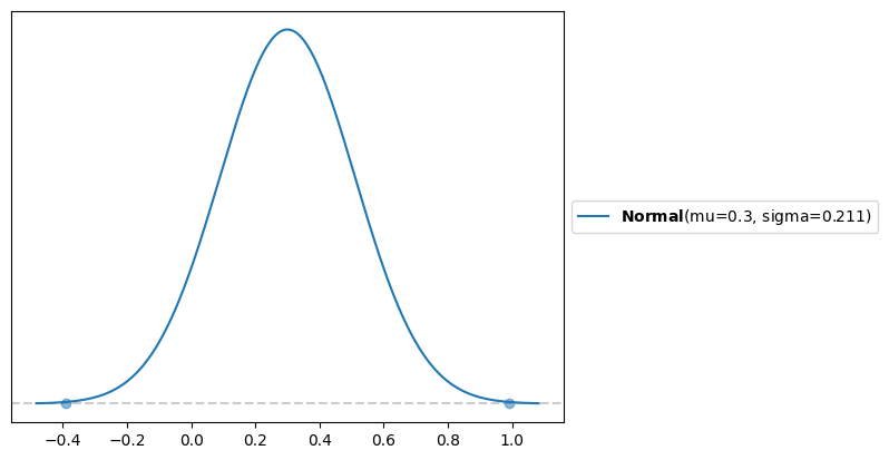
If we assume a Normal distribution between the bounds with mass of .999 we get
d = pl.unidimensional.maxent(pl.Normal(), lb, ub, .999)
1 - d[0].cdf(0)

which has the expected mean, 92% of the mass is above 0, so we are fairly certain of positive correlation.
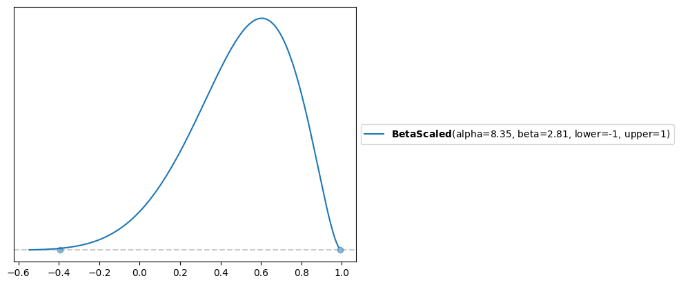
If we assume a BetaScaled we get a different shape
d2 = pl.unidimensional.maxent(pl.BetaScaled(lower=-1, upper=1), lb, ub, .999)
d2[0].mean()
1 - d2[0].cdf(0)

The mean of it is 0.5, and 96% of the mass > 0.